Study of Car Accidents in the United States

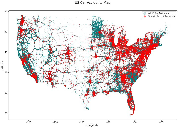
We chose to work with a set of United States car accident data from 2016 - 2020. The data set consists of ~3.5 million samples, each of which has 49 features.

Exploratory Data Analysis

The goal of this analysis is to assess the cleanliness and consistency of the data in order to engineer features that can be used to train a predictor of accident severity. To this end, we systematically explore the features and their relationships with other features using both summary statistics and visualizations. Please see the Google Colab notebook for further EDA.

Machine Learning

Under the scope of this project, we chose to perform our severity prediction for Pennsylvania state. Given that this is a multi-class classification problem, we have several algorithms to consider. Let’s look at each of them and see how they perform with the PA subset.

XGBoost is the winner here. XGBoost is a gradient boosting method, one of the best algorithms for classification problems. It handles large sized datasets very well with good execution speed. It can automatically handle missing values and apply regularized boosting method, thus it’s less prone to overfitting. It also does pruning for you. As a matter of fact, XGBoost is a frequent winner in a lot of Kaggle competitions.

Come very close is LightGBM. Light GBM is a fast, distributed, high-performance gradient boosting framework based on decision tree algorithm. It is capable of performing equally good with large datasets with a significant reduction in training time as compared to XGBoost.

Deep Learning

We attempt to predict the level of severity using the accident descriptions. We will use a Long Short Term Memory (LSTM) recurrent neural net (RNN) model for this task.

LSTM Introduction

The accident description is a form of sequential information. Intuitively, RNNs have memory that “captures” what have been calculated so far i.e. what happened in the last sentence will impact what happened in the next sentense. We then use these information to predict the “label” of the accident severity, i.e. category level 1 through 4. The architecture of the recurrent neural networks is below:

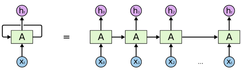
A chunk of neural network, “A”, looks at some input x(t) and outputs a value h(t). X(t) could be a word or a sentence, and h(t) is the probability of the next word or next sentence.

So how does that relate to our task of predicting accident severity given the description?

• We input a word or words of the description to the model
• At the end of each description, we give the model the label i.e. the severity category value
• RNNs, by passing input from last output, are able to retain information and able to leverage all these information at the end to make a severity prediction given a new accident description.

This works well for short descriptions but when we have to deal with a long descriptions, there will be a long term dependency problem. Therefore, we generally do not use vanilla RNNs, and we use Long Short Term Memory instead.

LSTM is a type of RNNs that can solve the long term dependency problem.

For this classification problem, we will use the many-to-one relationship model. The input are sequences of words, and the output is one single label, the accident severity.

Model Training

• The first layer is the embedded layer that uses 100 length vectors to represent each word.
• The next layer is the LSTM layer with 100 memory units.
• The output layer creates 4 output values, one for each category.
• Activation function is softmax for multi-class classification.
• Because it is a multi-class classification problem, categorical_crossentropy is used as the loss function.
• We use Adam optimization, which is an adaptive learning rate optimization algorithm that’s been designed specifically for training deep neural networks.
• We also implement 2 regularization methods to prevent overfitting, which are dropout (at 20%) and early stopping.

Epoch 1/10
633/633 [==============================] - 1076s 2s/step - loss: 0.3712 - accuracy: 0.8764 - val_loss: 0.2969 - val_accuracy: 0.9033
Epoch 2/10
633/633 [==============================] - 1091s 2s/step - loss: 0.2867 - accuracy: 0.9077 - val_loss: 0.2827 - val_accuracy: 0.9062
Epoch 3/10
633/633 [==============================] - 1076s 2s/step - loss: 0.2769 - accuracy: 0.9095 - val_loss: 0.2809 - val_accuracy: 0.9062
Epoch 4/10
633/633 [==============================] - 1073s 2s/step - loss: 0.2726 - accuracy: 0.9101 - val_loss: 0.2785 - val_accuracy: 0.9062
Epoch 5/10
633/633 [==============================] - 1073s 2s/step - loss: 0.2688 - accuracy: 0.9105 - val_loss: 0.2765 - val_accuracy: 0.9073
Epoch 6/10
633/633 [==============================] - 1071s 2s/step - loss: 0.2655 - accuracy: 0.9105 - val_loss: 0.2757 - val_accuracy: 0.9076
Epoch 7/10
633/633 [==============================] - 1071s 2s/step - loss: 0.2635 - accuracy: 0.9112 - val_loss: 0.2767 - val_accuracy: 0.9071
Epoch 8/10
633/633 [==============================] - 1073s 2s/step - loss: 0.2626 - accuracy: 0.9118 - val_loss: 0.2693 - val_accuracy: 0.9087
Epoch 9/10
633/633 [==============================] - 1074s 2s/step - loss: 0.2597 - accuracy: 0.9115 - val_loss: 0.2698 - val_accuracy: 0.9089
Epoch 10/10
633/633 [==============================] - 1073s 2s/step - loss: 0.2584 - accuracy: 0.9125 - val_loss: 0.2716 - val_accuracy: 0.9076

Using just 50,000 sample records (over 3.5 millions available records), we can achieve an accuracy of 91.1% with recurrent neural nets. This already beats almost all of our classical ML models. The downside is that it takes a long time to train our LSTM model.